PrePost

Connecting to the database

First, generate the artificial data (sqlite files for each database), as follows:

library(PrePost)

# generate example databases
prepost_example()

This will create a folder called gendata in your working directory, containing the database files for the example cohort. Next, you can connect to this databases using:

library(PrePost)
library(dplyr)
library(icdb)

# connect to ICB server using this
# srv <- icdb::server("[data_source_name]"])  #see ICDB documentation for details

# in this example we can connect to the synthetic data using
srv <- example_server()

Define the cohort

Here an example cohort is provided on the example server. All we need is the (pseudo) NHS number and the datetime of interest.

ids  <- srv$cohort$COHORT_SYNTH %>% select(nhs_number) %>% pull()
date <- srv$cohort$COHORT_SYNTH %>% select(index_event_time) %>% pull() %>% as.POSIXct()

Define the activity filters

Here we must decide which healthcare activity we are interested in. We can define any number of filters to act on SWD activity columns, as a named list. The name of each filter will be used in the subsequent plots.

activity_filter <- list(
  "A+E"                 = "pod_l1=='secondary' & pod_l2a=='ae'",
  "Community in-person" = "pod_l1=='community' & pod_l3=='physical'",
  "999"                 = "pod_l1=='999'",
  "111"                 = "pod_l1=='111'",
  "GP"                  = "pod_l1=='primary_care_contact'"
)

Create the PrePost object

Next we create a PrePost object, defining the window of interest. If working on the ICB servers you will need to pass the name of your ICB data source as the parameter srv_name. Please see the ICDB package documentation for instructions on how to setup the ICB data source. In this example we directly pass an example_server - this is purely for demonstration.

obj <- PrePost(nhs_number       = ids,
               index_event_time = date,
               window_pre       = 31,
               window_post      = 30, 
               window_units     = "days",
               activity_filter  = activity_filter,
               svr              = example_server(), 
               svr_name         = NA_character_)

Descriptives

Run the descriptive analysis

run_descriptives(obj)

Activity analysis

Run the activity analysis

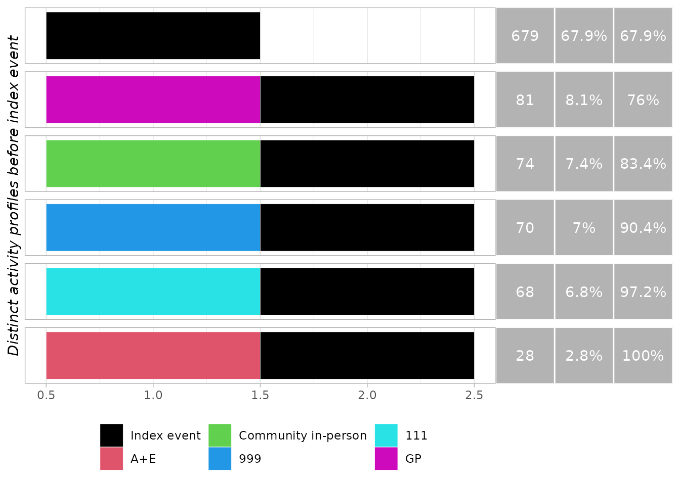
run_activity_summary(obj, "before")

Summary of activity volumes before the index event

Activity	Mean activity per instance	Instances with >0 activity	Mean activity per instance with >0 activity
111	0.07	6.8%	1
999	0.07	7%	1
A+E	0.03	2.8%	1
Community in-person	0.07	7.4%	1
GP	0.08	8.1%	1

run_activity_summary(obj, "after")

Summary of activity volumes after the index event

Activity	Mean activity per instance	Instances with >0 activity	Mean activity per instance with >0 activity
111	0.07	7.2%	1
999	0.09	9.2%	1
A+E	0.02	2.3%	1
Community in-person	0.06	6.2%	1
GP	0.08	7.7%	1

Theographs

Generate the theographs

generate_theographs(obj)

Activity volume

Analyse the activity volume

run_activity_volume(obj, "before")
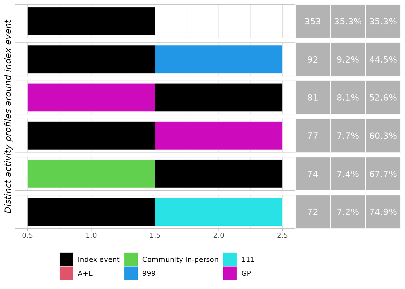
run_activity_volume(obj, "after")

Trace plots

Generate the trace plots

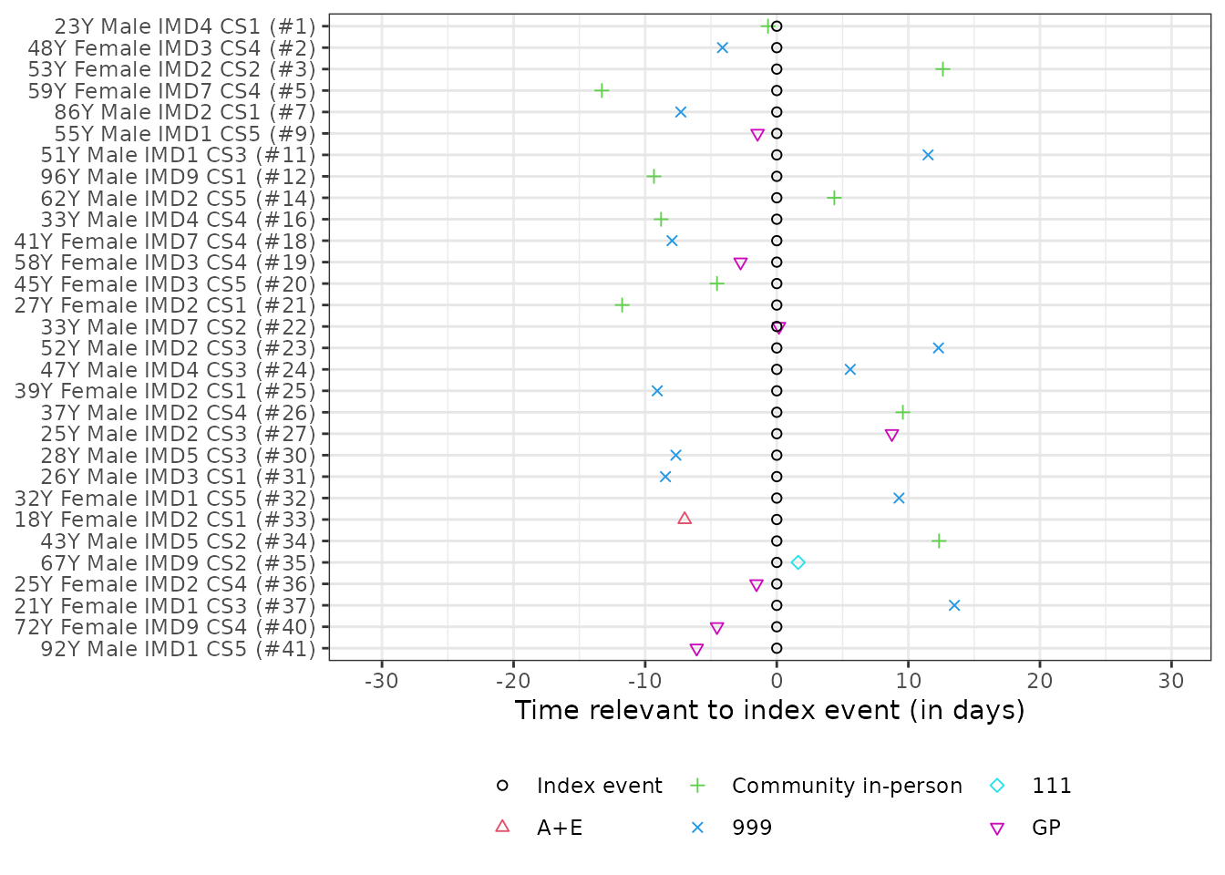
generate_trace_plots(obj, "before")

generate_trace_plots(obj, "before")

generate_trace_plots(obj, "around")